9. Results Visualization#
The Results toolbar groups the tools for selecting result states and displaying result plots.
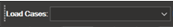
The load case selector displays all load cases associated with the model, allowing you to select the specific load case to analyze.
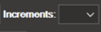
The increments selector shows the different increments available within the selected load case, enabling you to choose the increment for detailed examination.
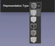
NaxToView displays different types of results through separate plot windows, each with its own configuration. From each window, you can manage results, components, sections, coordinate system, and scalar bar settings independently, allowing full simultaneous control over multiple visualizations.

9.1. Contour Plot#
The Contour Plot window represents scalar results as contours on the model geometry.
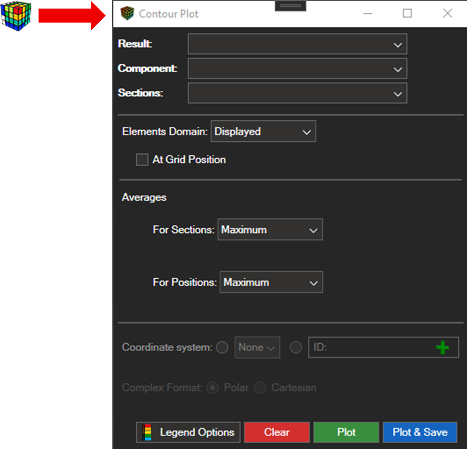
9.1.1. Result Options#
Result: Selects the result to display (stresses, strains, displacements, etc.).
Component: Determines the specific component of the result (XX, YY, ZZ, etc.).
Sections: Selects the section or range of sections on which the result is plotted.
9.1.2. Domain#
Elements Domain: Defines whether the contour is drawn over visible elements, selected elements, or a user-defined element set.
At Grid Position: Displays the result value at the nodal position. Use this option when results are computed at integration points and an extrapolated nodal value is required for display.
9.1.3. Averages#
Controls how results are handled when multiple points exist per element:
For Sections: Choose between Maximum, Minimum, or Average.
For Positions: Select the desired value when the element has multiple integration points.
9.1.4. Coordinate System#
Selects the coordinate system in which the result is displayed. Options include the global system, the element local system, or a user-defined coordinate system.
9.1.5. Complex Results#
When the result is complex, the following options are enabled:
Polar → Magnitude or Phase
Cartesian → Real or Imaginary
9.1.6. Legend Options#
Opens the scalar bar configuration associated exclusively with this plot. See Section 9.4. Scalar Bar Options for more details.
9.1.7. Plot & Save#
The Plot & Save button allows you to plot a result and automatically save its state for later reuse.
Integration with the Session Tree
When this feature is used, a new entry is created in the Session Tree, located within the active Window and the corresponding View. Each saved result is added as a new node in the session tree (see 7. Session Tree).
Interacting with saved plots
Right-clicking a saved plot provides the following actions:
Activate — re-plots the stored result on exactly the same elements as originally selected.
Delete — removes the saved plot from the Session Tree.
This functionality allows you to store different result representation states and easily retrieve them later, without having to repeat the selection or the previous configuration.
9.2. Vector Plot#
The Vector Plot window represents vector results using arrows, such as displacements, velocities, forces, or rotations.
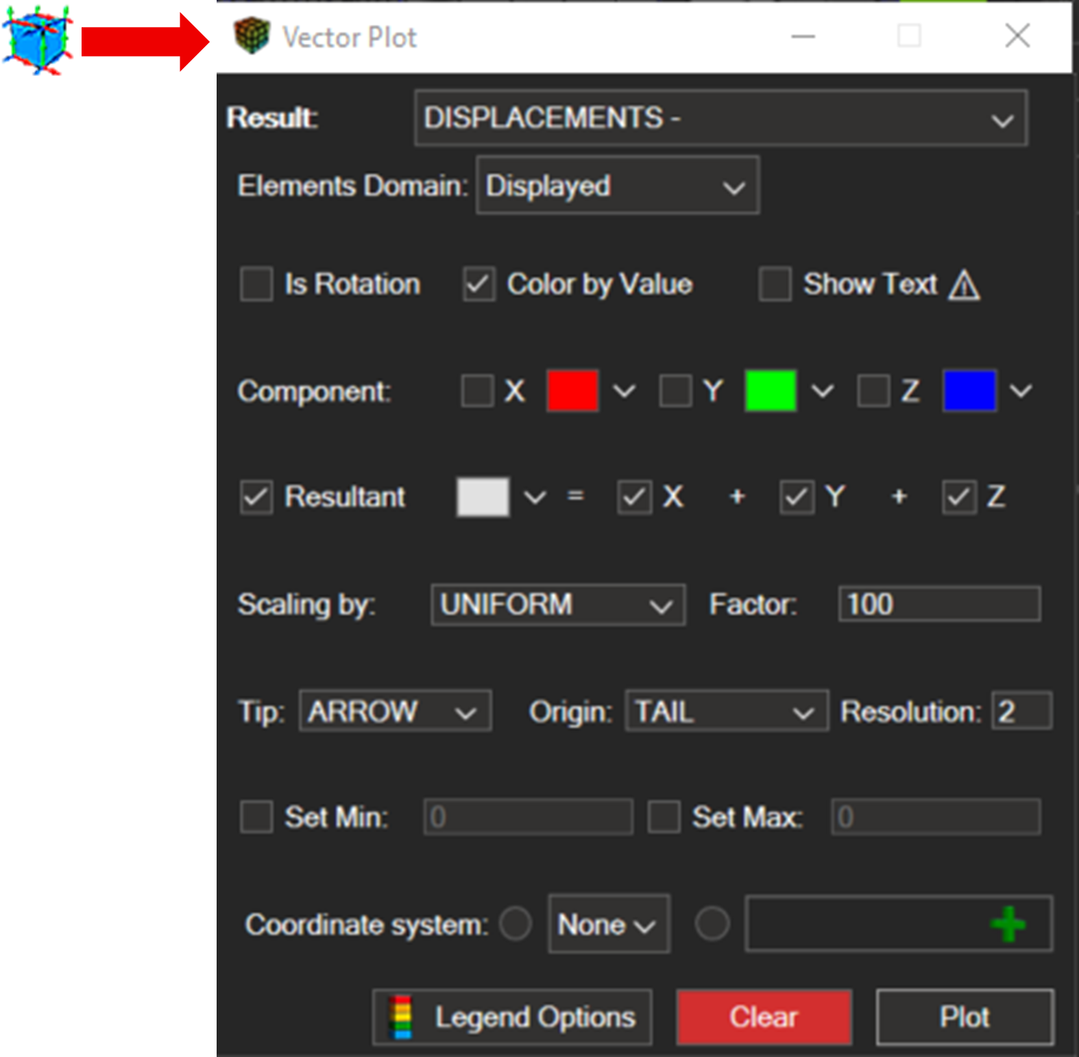
9.2.1. Main Options#
Result: Selects the vector field to display.
Elements Domain: Determines which elements the vectors are drawn on.
Is Rotation: Interprets the components as rotations (Rx, Ry, Rz) instead of displacements.
9.2.2. Colors and Labels#
Color by Value: Colours vectors according to their magnitude.
Show Text: Displays a label with the vector value.
9.2.3. Components#
Components are selected directly in the plot window:
X, Y, Z → Individual representation
Resultant → Combined magnitude of the selected components
9.2.4. Scaling#
Auto: Automatically determined scale factor.
By Value: Vector length proportional to its value.
Uniform: All vectors have the same length.
Factor: Allows manual scale adjustment.
9.2.5. Geometric Options#
Tip: Sets the vector arrowhead style (arrow or none).
Origin: Starting point of the vector.
Resolution: Controls the polygon count of the rendered vectors. Higher values produce smoother arrows at the cost of rendering performance.
9.2.6. Filters#
Set Min / Set Max: Only vectors within the defined value range are displayed.
9.2.7. Coordinate System#
Selects the reference system for vector representation.
9.2.8. Legend Options#
Configures the scalar bar used in this vector plot. See Section 9.4. Scalar Bar Options for more details.
9.3. Tensor Plot#
The Tensor Plot represents tensor quantities — such as stresses or strains — showing both axial and shear components.
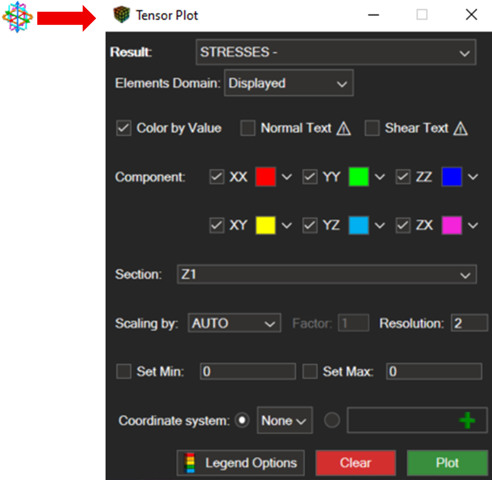
9.3.1. Main Options#
Result: Defines the tensor to display.
Elements Domain: Determines the domain of elements used for visualisation.
9.3.2. Coloring and Labels#
Color by Value: Colours tensors according to their value.
Normal Text: Displays labels for axial values XX, YY, ZZ.
Shear Text: Displays shear values XY, YZ, ZX.
9.3.3. Components#
Activate individual axial and shear components and assign a colour to each.
9.3.4. Section#
Selects the section of the tensor to visualise.
9.3.5. Scaling#
Auto: Automatic scaling based on magnitude.
By Value: Size depends on the tensor value.
Uniform: All tensors have the same scale.
Factor: Manual adjustment.
9.3.6. Geometric Options#
Tip: Tensor head style (arrow or none).
Origin: Origin point of the representation.
Resolution: Controls the polygon count of the rendered tensor glyphs.
9.3.7. Filters#
Set Min / Set Max: Controls which tensors are displayed according to their value.
9.3.8. Coordinate System#
Selects the reference system for tensor representation.
9.3.9. Legend Options#
Opens the scalar bar configuration associated exclusively with this tensor plot. See Section 9.4. Scalar Bar Options for more details.
9.4. Scalar Bar Options#
The Scalar Bar has been redesigned to improve both usability and customisation of result visualisation. It is now fully interactive: values and colours can be modified directly from the 3D viewport, without needing to open a separate configuration window.
9.4.1. Interactive Editing#
The Scalar Bar supports direct editing in two ways:
Double-click on a value — opens an inline editor to change that scale value directly on the bar.
Double-click on a colour — opens a colour picker to replace that colour swatch.
Additionally, right-clicking on the Scalar Bar opens the options window, from which scale values and all other settings can also be edited.
9.4.2. Options Window#
Click the scalar bar icon in the toolbar or right-click the Scalar Bar to open the options window.
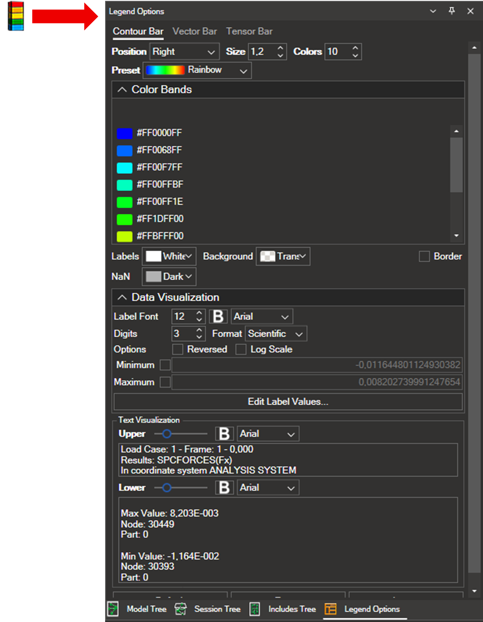
The options window has been updated to facilitate editing of scale intervals and improve the overall user experience. The available settings are organised as follows.
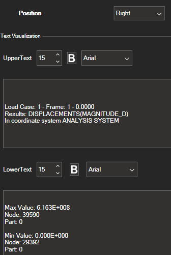
Position and font
You can adjust the position of the legend (left or right) and customise the font size and style.
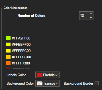
Colour options
The number of colours shown in the legend.
Customise individual colours by clicking on a colour swatch and selecting from the colour picker.
The colour of the text, the background of the text box, and the border of the text box.
Colour theme — select a predefined colour theme to change the default colours used by the Scalar Bar.
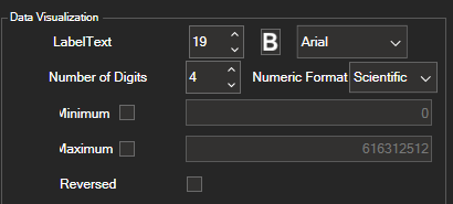
Display settings
Font size and style
Number of significant digits for each value
Numeric format
Maximum and minimum value range
Invert the legend colours
9.4.3. Logarithmic Interpolation#
The Scalar Bar now supports logarithmic interpolation for the scale values. When enabled, the intervals between values follow a logarithmic distribution instead of a linear one. This is particularly useful for results that span several orders of magnitude, as it provides better visual resolution in the lower range of the scale.
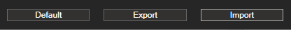
9.4.4. Export and Import#
The legend configuration can be saved for future use. To save the configuration, click Export, then choose a location and filename for the .xml file. To reuse a saved configuration, click Import and select the file. To restore defaults, click Defaults.
9.5. Clear Plot#

Click the Clear Plot icon to remove the active result plot from the 3D view.
9.6. Deformed Settings#
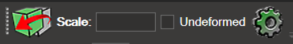
The Deformed Settings toolbar controls the display of the model’s deformed shape.
Enter the scale factor in the Deformation field.

Click the icon to display the deformed shape; click it again to clear it.
Select Undeformed to overlay the undeformed mesh on the deformed model in the 3D view. The option can be toggled at any time.
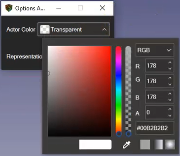
Clicking the settings icon opens the Undeformed Mesh properties window.
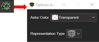
You can select the mesh colour.
Select the rendering style for the undeformed mesh:
Opaque
Opaque Wireframe
Transparent
Transparent Wireframe
Opaque Feature Edges