3. Loading Model and Results Data

NaxToView provides several methods for loading model and results data. This section describes the available import options and provides step-by-step guidance for loading your files.

3.1. Import Options

The File → Import submenu offers different import options depending on your needs:

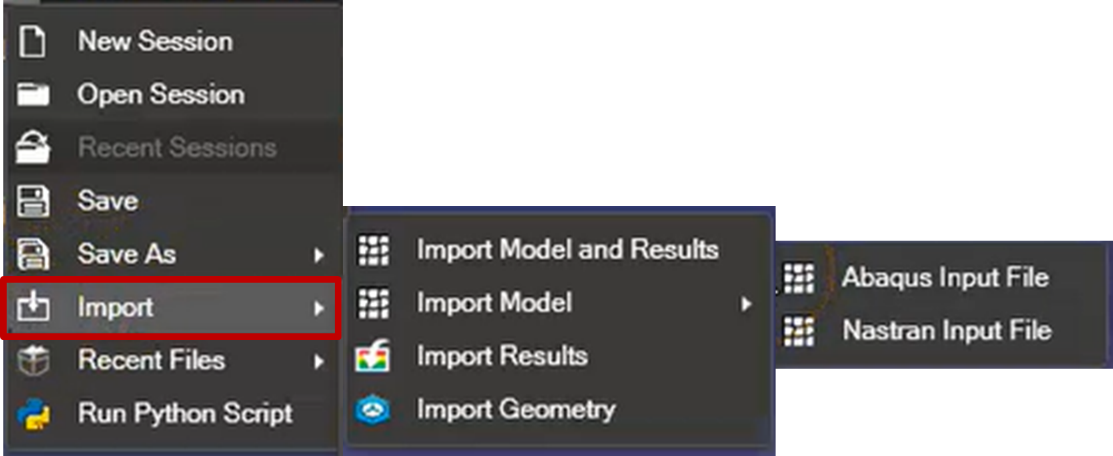
The following table summarizes the available import options and their supported file formats:

Import Option	Purpose	Supported Formats
Import Model and Results	Loads both the model mesh and results	*.op2, *.xdb, *.h5, *.h3d, *.odb, *.rst
Import Model	Loads only the mesh, without results	*.bdf, *.dat, *.inp, *.inc, or any other text format for Nastran, Abaqus, Ansys or Optistruct input files
Import Results	Loads results for an already-loaded model	*.op2, *.xdb, *.h5, *.h3d, *.odb, *.rst
Import Geometry	Loads surface geometry	*.stl

3.1.1. Import Model and Results

Loads both the model mesh and results from binary output files. This is the most common import option for post-processing analysis results.

Supported formats: *.op2, *.xdb, *.hdf5, *.h3d, *.odb, *.rst

3.1.2. Import Model

Imports only the model mesh, without results. Use this option when you want to inspect the model geometry or when results are not yet available.

Supported input formats: *.bdf, *.dat (Nastran), *.inp (Abaqus)

3.1.3. Import Results

Imports results in HDF5 format for a model that has already been loaded. This option is useful when you want to load additional result sets for an existing model.

Supported format: *.hdf5

For more information about the NaxTo HDF5 format, see 22. NaxTo HDF5 Format.

3.1.4. Import Geometry

Imports surface geometry from STL files. Use this option to load geometric representations without finite element mesh data.

Supported format: *.stl

3.1.5 Import Coordinate Systems from CSV

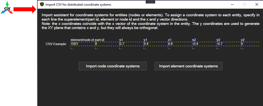
This tool is very useful when you need to work with results in independent coordinate systems for each entity (node/element), as it allows you to load a CSV with a list of systems.

To do so, click on the icon and a window with an import wizard will appear.

Select the type of entity to be loaded (element or node) and select the csv file.

An example of the csv is the one that follows:

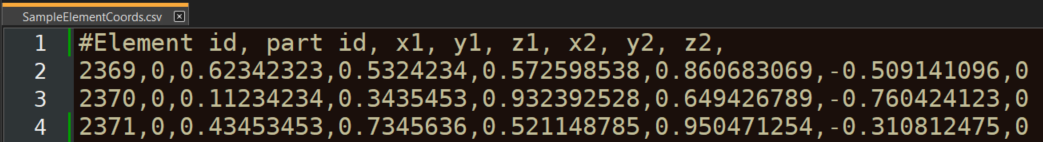
Fields are split by commas, and coordinates use a decimal point. The first line is an example of a comment, that begins with a #.

The coordinate systems are defined with the following fields:

• ID: of the element/node that is being defined

• Part ID: of the superelement of the element/node. Default: 0.

• x1, y1, z1: coordinates of the first vector

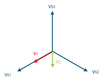
• x2, y2, z2: coordinates of a vector contained in the XY plane of the system. Note that this vector not only defines the plane, but also the direction of the second and third vector (the scalar product of this vector and the vector 2 of the defined coordinate system is always positive).

For example, if the line contains the vector v1 and v2, the generated coordinate system would be S = {vS1, vS2, vS3}

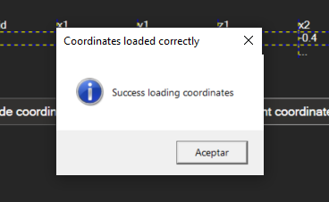
If the format is correct and the “ActiveMessageBox” option is marked in the user options, a success message will pop up.

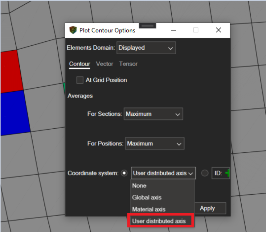
From now on, a new output coordinate system will appear on the plot contour options for supported results.

3.2. Import Recent Files

The File → Import Recent Files submenu provides quick access to recently opened files, streamlining your workflow.

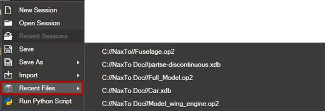
The list displays the most recently opened files. Click a file path to load it immediately without navigating through the file browser.

3.3. Loading a Model: Step-by-Step

To load a model with results:

1. Click File → Import → Import Model and Results.

2. In the file browser, navigate to your results file (e.g., model.op2, model.odb).

3. Select the file and click Open.

4. NaxToView reads the file and displays a progress indicator.

5. Once loading is complete, the model appears in the 3D viewport.

6. The Model Tree populates with the model structure (elements, properties, materials, etc.).

If results data is available, you can visualize them using the Results toolbar (see 9. Results Visualization).

Note

Large models may take several minutes to load. The progress indicator shows the current loading status.

3.4. What Happens After Import

After successfully importing a file:

• The model displays in the 3D viewport with default visualization settings

• The Model Tree shows the model hierarchy organized by entities, properties, materials, parts, and coordinate systems

• If results were imported, the Results panel becomes available with result types (displacements, stresses, etc.)

• The Session Tree shows the active window and view configuration

• If the file contained multiple load cases or time steps, they appear in the results selector

You can now navigate the model, apply visualization settings, and analyze results as described in the following sections.