N2PGetLoadFasteners User Manual

Overview

N2PGetLoadFasteners is a NaxToPy module which provides information about the loads that fasteners in a model experience. It must be used after the N2PGetFasteners class, since it makes use of joints created using that class.

Example Usage

In order to use the program, the user should call the N2PGetFasteners class, as explained in its corresponding documentation, and then basically call all functions previously explained. Several examples will be given in order to accurately represent most of the ways that this program can be used.

After all necessary fasteners have been obtained, the user should create the N2PGetLoadFasteners instance and load them:

import NaxToPy as n2p
from NaxToPy.Modules.Fasteners.N2PGetFasteners import N2PGetFasteners
from NaxToPy.Modules.Fasteners.N2PGetLoadFasteners import N2PGetLoadFasteners

model = n2p.load_model(r"C:\user\models\FEMModel.fem")

fasteners = N2PGetFasteners()
fasteners.Model = model
fasteners.calculate()

loads = N2PGetLoadFasteners()
loads.GetFasteners = fasteners

The same thing could have been done in the following way:

import NaxToPy as n2p
from NaxToPy.Modules.Fasteners.N2PGetFasteners import N2PGetFasteners
from NaxToPy.Modules.Fasteners.N2PGetLoadFasteners import N2PGetLoadFasteners

model = n2p.load_model(r"C:\user\models\FEMModel.fem")

fasteners = N2PGetFasteners()
fasteners.Model = model
fasteners.calculate()

loads = N2PGetLoadFasteners()
loads.Model = model
loads.ListJoints = fasteners.JointsList

Now, the user should load the results files. Consider the case when the user only wants to load one file:

import NaxToPy as n2p
from NaxToPy.Modules.Fasteners.N2PGetFasteners import N2PGetFasteners
from NaxToPy.Modules.Fasteners.N2PGetLoadFasteners import N2PGetLoadFasteners

model = n2p.load_model(r"C:\user\models\FEMModel.fem")

fasteners = N2PGetFasteners()
fasteners.Model = model
fasteners.calculate()

loads = N2PGetLoadFasteners()
loads.GetFasteners = fasteners
loads.ResultsFiles = r"C:\user\models\ResultsFiles.op2"

In this point, a new model would be created. Consider now the case when the user wants to load several results files:

import NaxToPy as n2p
from NaxToPy.Modules.Fasteners.N2PGetFasteners import N2PGetFasteners
from NaxToPy.Modules.Fasteners.N2PGetLoadFasteners import N2PGetLoadFasteners

model = n2p.load_model(r"C:\user\models\FEMModel.fem")

fasteners = N2PGetFasteners()
fasteners.Model = model
fasteners.calculate()

loads = N2PGetLoadFasteners()
loads.GetFasteners = fasteners
loads.ResultsFiles = [
    r"C:\user\models\ResultsFiles1.op2",
    r"C:\user\models\ResultsFiles2.op2"
]

Finally, let us consider the case when the user wants to load a folder full of results files:

import NaxToPy as n2p
from NaxToPy.Modules.Fasteners.N2PGetFasteners import N2PGetFasteners
from NaxToPy.Modules.Fasteners.N2PGetLoadFasteners import N2PGetLoadFasteners

model = n2p.load_model(r"C:\user\models\FEMModel.fem")

fasteners = N2PGetFasteners()
fasteners.Model = model
fasteners.calculate()

loads = N2PGetLoadFasteners()
loads.GetFasteners = fasteners
loads.ResultsFiles = r"C:\user\models\ResultsFiles"

After results have been loaded, the user could use all default parameters and obtain the results (take note that, if no diameters have been selected, bypass loads will not be calculated):

import NaxToPy as n2p
from NaxToPy.Modules.Fasteners.N2PGetFasteners import N2PGetFasteners
from NaxToPy.Modules.Fasteners.N2PGetLoadFasteners import N2PGetLoadFasteners

model = n2p.load_model(r"C:\user\models\FEMModel.fem")

fasteners = N2PGetFasteners()
fasteners.Model = model
fasteners.calculate()

loads = N2PGetLoadFasteners()
loads.GetFasteners = fasteners
loads.ResultsFiles = r"C:\user\models\ResultsFiles.op2"
loads.get_model()
loads.get_results_joints()
loads.get_forces_joints()
loads.get_bypass_joints()

This could have been done in an easier way:

import NaxToPy as n2p
from NaxToPy.Modules.Fasteners.N2PGetFasteners import N2PGetFasteners
from NaxToPy.Modules.Fasteners.N2PGetLoadFasteners import N2PGetLoadFasteners

model = n2p.load_model(r"C:\user\models\FEMModel.fem")

fasteners = N2PGetFasteners()
fasteners.Model = model
fasteners.calculate()

loads = N2PGetLoadFasteners()
loads.GetFasteners = fasteners
loads.ResultsFiles = r"C:\user\models\ResultsFiles.op2"
loads.get_model()
loads.get_results_joints()
loads.get_analysis_joints()

And also in an even easier way:

import NaxToPy as n2p
from NaxToPy.Modules.Fasteners.N2PGetFasteners import N2PGetFasteners
from NaxToPy.Modules.Fasteners.N2PGetLoadFasteners import N2PGetLoadFasteners

model = n2p.load_model(r"C:\user\models\FEMModel.fem")

fasteners = N2PGetFasteners()
fasteners.Model = model
fasteners.calculate()

loads = N2PGetLoadFasteners()
loads.GetFasteners = fasteners
loads.ResultsFiles = r"C:\user\models\ResultsFiles.op2"
loads.calculate()

In order to assign joints a diameter, this can be done in two ways. Firstly, they could be manually assigned:

import NaxToPy as n2p
from NaxToPy.Modules.Fasteners.N2PGetFasteners import N2PGetFasteners
from NaxToPy.Modules.Fasteners.N2PGetLoadFasteners import N2PGetLoadFasteners

model = n2p.load_model(r"C:\user\models\FEMModel.fem")

fasteners = N2PGetFasteners()
fasteners.Model = model
fasteners.calculate()

loads = N2PGetLoadFasteners()
loads.GetFasteners = fasteners
loads.ResultsFiles = r"C:\user\models\ResultsFiles.op2"

fasteners.ListJoints[0].Diameter = 4.2
fasteners.ListJoints[1].Diameter = 4.2

for joint in fasteners.JointsList[2:]:
    joint.Diameter = 4.5

loads.calculate()

Alternatively, diameters could have been automatically assigned by using the default diameter attributes:

import NaxToPy as n2p
from NaxToPy.Modules.Fasteners.N2PGetFasteners import N2PGetFasteners
from NaxToPy.Modules.Fasteners.N2PGetLoadFasteners import N2PGetLoadFasteners

model = n2p.load_model(r"C:\user\models\FEMModel.fem")

fasteners = N2PGetFasteners()
fasteners.Model = model
fasteners.calculate()

loads = N2PGetLoadFasteners()
loads.GetFasteners = fasteners
loads.ResultsFiles = r"C:\user\models\ResultsFiles.op2"
loads.DefaultDiameter = 4.2
loads.calculate()

The user could have also manually altered the “AdjacencyLevel” attribute, which controls how many elements will be loaded in the “get_model” method:

import NaxToPy as n2p
from NaxToPy.Modules.Fasteners.N2PGetFasteners import N2PGetFasteners
from NaxToPy.Modules.Fasteners.N2PGetLoadFasteners import N2PGetLoadFasteners

model = n2p.load_model(r"C:\user\models\FEMModel.fem")

fasteners = N2PGetFasteners()
fasteners.Model = model
fasteners.calculate()

loads = N2PGetLoadFasteners()
loads.GetFasteners = fasteners
loads.AdjacencyLevel = 3
loads.ResultsFiles = r"C:\user\models\ResultsFiles.op2"
loads.calculate()

The previous cases assumed that the user wanted to analyse all load cases in the model. Consider the case when they only want to analyse a certain amount of them, whose IDs are known:

import NaxToPy as n2p
from NaxToPy.Modules.Fasteners.N2PGetFasteners import N2PGetFasteners
from NaxToPy.Modules.Fasteners.N2PGetLoadFasteners import N2PGetLoadFasteners

model = n2p.load_model(r"C:\user\models\FEMModel.fem")

fasteners = N2PGetFasteners()
fasteners.Model = model
fasteners.calculate()

loads = N2PGetLoadFasteners()
loads.GetFasteners = fasteners
loads.ResultsFiles = r"C:\user\models\ResultsFiles.op2"
loads.LoadCases = loads.Model.get_load_case(253, 333, 10001)
loads.calculate()

The previous cases also assumed that the results did not include data in their corners. If the user is certain that all of them do (an error will appear if some of them do not), they could obtain more precise results:

import NaxToPy as n2p
from NaxToPy.Modules.Fasteners.N2PGetFasteners import N2PGetFasteners
from NaxToPy.Modules.Fasteners.N2PGetLoadFasteners import N2PGetLoadFasteners

model = n2p.load_model(r"C:\user\models\FEMModel.fem")

fasteners = N2PGetFasteners()
fasteners.Model = model
fasteners.calculate()

loads = N2PGetLoadFasteners()
loads.GetFasteners = fasteners
loads.ResultsFiles = r"C:\user\models\ResultsFiles.op2"
loads.CornerData = True
loads.calculate()

Consider the case when the user wants to modify some bypass parameters, for example, the projection tolerance, the maximum number of iterations and the material factor of composite materials:

import NaxToPy as n2p
from NaxToPy.Modules.Fasteners.N2PGetFasteners import N2PGetFasteners
from NaxToPy.Modules.Fasteners.N2PGetLoadFasteners import N2PGetLoadFasteners

model = n2p.load_model(r"C:\user\models\FEMModel.fem")

fasteners = N2PGetFasteners()
fasteners.Model = model
fasteners.calculate()

loads = N2PGetLoadFasteners()
loads.GetFasteners = fasteners
loads.ResultsFiles = r"C:\user\models\ResultsFiles.op2"
loads.BypassParameters = {
    "projection tolerance": 0.1,
    "MAX ITERATIONS": 50,
    "Material Factor composite": 4.0
}
loads.calculate()

Take note that it is not relevant it the bypass parameters are written in upper case, lower case or a combination of both. Consider the case when the user wants to modify the number of load cases that will be analysed on each iteration:

import NaxToPy as n2p
from NaxToPy.Modules.Fasteners.N2PGetFasteners import N2PGetFasteners
from NaxToPy.Modules.Fasteners.N2PGetLoadFasteners import N2PGetLoadFasteners

model = n2p.load_model(r"C:\user\models\FEMModel.fem")

fasteners = N2PGetFasteners()
fasteners.Model = model
fasteners.calculate()

loads = N2PGetLoadFasteners()
loads.GetFasteners = fasteners
loads.ResultsFiles = r"C:\user\models\ResultsFiles.op2"
loads.LoadCaseNumber = 200
loads.calculate()

Consider now the case when the user wants to change the type of analysis to the Altair style:

import NaxToPy as n2p
from NaxToPy.Modules.Fasteners.N2PGetFasteners import N2PGetFasteners
from NaxToPy.Modules.Fasteners.N2PGetLoadFasteners import N2PGetLoadFasteners

model = n2p.load_model(r"C:\user\models\FEMModel.fem")

fasteners = N2PGetFasteners()
fasteners.Model = model
fasteners.calculate()

loads = N2PGetLoadFasteners()
loads.GetFasteners = fasteners
loads.ResultsFiles = r"C:\user\models\ResultsFiles.op2"
loads.TypeAnalysis = "Altair"
loads.calculate()

Consider now the case when the user wants to export the obtained PAG results to a CSV file:

import NaxToPy as n2p
from NaxToPy.Modules.Fasteners.N2PGetFasteners import N2PGetFasteners
from NaxToPy.Modules.Fasteners.N2PGetLoadFasteners import N2PGetLoadFasteners

model = n2p.load_model(r"C:\user\models\FEMModel.fem")

fasteners = N2PGetFasteners()
fasteners.Model = model
fasteners.calculate()

loads = N2PGetLoadFasteners()
loads.GetFasteners = fasteners
loads.ResultsFiles = r"C:\user\models\ResultsFiles.op2"
loads.ExportLocation = r"C:\user\models"
loads.TypeExport = "PAG_CSV"
loads.calculate()

In the previous case, the file would be named in the default way, but this can be changed by the user:

import NaxToPy as n2p
from NaxToPy.Modules.Fasteners.N2PGetFasteners import N2PGetFasteners
from NaxToPy.Modules.Fasteners.N2PGetLoadFasteners import N2PGetLoadFasteners

model = n2p.load_model(r"C:\user\models\FEMModel.fem")

fasteners = N2PGetFasteners()
fasteners.Model = model
fasteners.calculate()

loads = N2PGetLoadFasteners()
loads.GetFasteners = fasteners
loads.ResultsFiles = r"C:\user\models\ResultsFiles.op2"
loads.AnalysisName = "New analysis"
loads.ExportLocation = r"C:\user\models"
loads.TypeExport = "PAG_CSV"
loads.calculate()

Results

After having analysed all joints, the user could want to obtain some information out of them in the console. In this example, only some of the properties are called, but more information could be extracted:

import NaxToPy as n2p
from NaxToPy.Modules.Fasteners.N2PGetFasteners import N2PGetFasteners
from NaxToPy.Modules.Fasteners.N2PGetLoadFasteners import N2PGetLoadFasteners
model = n2p.load_model(r"C:\user\models\FEMModel.fem")
fasteners = N2PGetFasteners()
fasteners.Model = model
fasteners.calculate()
loads = N2PGetLoadFasteners()
loads.GetFasteners = fasteners
loads.ResultsFiles = r"C:\user\models\ResultsFiles.op2"
loads.calculate()
joint1Plates = fasteners.JointsList[0].PlateList
joint2PartID = fasteners.JointsList[1].PartID
joint3Diameter = fasteners.JointsList[2].Diameter
attachment1Pitch = fasteners.AttachmentsList[0].Pitch
attachment2Plates = fasteners.AttachmentsList[1].AttachedPlatesList
joint3AttachmentID = fasteners.JointsList[2].Attachment.ID
bolt1ElementsIID = fasteners.BoltsList[0].ElementsInternalIDList
bolt2AxialForce = fasteners.BoltsList[1].AxialForce
bolt3Cards = fasteners.BoltsList[2].Cards
joint4BoltLoadAngle = fasteners.JointsList[3].Bolt.LoadAngle
plate1InternalID = fasteners.PlatesList[0].ID
plate2Force = fasteners.PlateList[1].BearingForce
plate3MxTotal = fasteners.PlateList[2].MxTotal
plate4Fluxes = fasteners.PlateList[3].BoxFluxes
joint5Plate2Normal = fasteners.JointsList[4].PlateList[1].Normal  

Class Breakdown

Class Properties

As explained before, N2PGetLoadFasteners is a NaxToPy class that provides information about the loads that fasteners in a model experience and, optionally, exports them. In order to calculate a fastener’s loads, the user must already have the fasteners loaded, which is done in the N2PGetFasteners class. The class has the following properties:

• ResultsFiles: list of strings (compulsory input) representing the results file(s) to be loaded. The user can load a single results file (as a string and not necessarily a list of strings), several results files (as a list of strings) or a folder full of results files (as a string representing the folder’s path). If a folder is loaded, then the results files inside it are extracted using the “import_results” method, which is located in N2PLoadModel. The program supports .op2, .xdb, .odb, .h5, .h3d, and .rst files. This is a compulsory input as long as the model loaded in the “Model” or “GetFasteners” attribute does not include results. If it does, this is not a compulsory input. This attribute must be either a list of strings or a single string, or an error will occur. An error will also occur if the folder path or the file path do not exist.

• GetFasteners: N2PGetFasteners object (compulsory input) that was calculated with the N2PGetFasteners class. If this is an input, then “JointsList” and “Model” are automatically filled, so they should not be inputs. This attribute must be a N2PGetFasteners instance, or an error will occur. If this attribute is set and the Model and/or the JointsList attributes have been previously set, a warning is displayed, for this list of joints and model will overwrite the ones that have been set before.

• JointsList: list of N2PJoint objects (compulsory input) to be analysed. If this is an input, then “Model” must also be an input and “GetFasteners” should not. This attribute must be a list, tuple or set of N2PJoint instances, or a single N2PJoint. In any case, it will be transformed into a list. If this attribute is not a list, tuple, set or N2PJoint, an error will occur. If any item of the list (or tuple, or set) are not N2PJoint instances, a warning will appear and they will be removed from the list. If the GetFasteners attribute has been filled in, a warning will show up, as this list will overwrite the one that had come from GetFasteners.

• Model: N2PModelContent object (compulsory input) defining the model with the load cases results already loaded. If this is an input, then “ListJoints” must also be an input and “GetFasteners” should not. This attribute must be a N2PModelContent instance, or an error will occur. If this attribute is set and the N2PGetFasteners attribute has been previously set, a warning is displayed, for the previous model will be overwritten.

• AdjacencyLevel: integer (non-compulsory input) representing the adjacency radius, that is, how many layers of adjacent elements (from the fasteners) are to be loaded in the new model. By default, it is set to four. This attribute must be an integer, or an error will occur.

• LoadCases: list of N2PLoadCase instances (non-compulsory input) representing the load cases to be analysed. This attribute could be set to be a list, tuple, set or a single N2PLoadCase. In any case, it will be transformed into a list. If this attribute is not set, all load cases in the model will be analysed. If this attribute is not a list, set or tuple of N2PLoadCase instances, or a single N2PLoadCase instance, an error will occur. It any item of the list (or tuple, or set) is not an N2PLoadCase, it will be removed from the list and a warning will appear.

• CornerData: Boolean (non-compulsory input) representing if the results in the model have information in the corners or not. By default, it is set to False, so no corner data will be used, even if it is present. This attribute must be a Boolean, or an error will occur.

• BypassParameters: dictionary (non-compulsory input) representing some parameters to be used in the bypass calculations. Those parameters, with their default values, are the following:

  • MATERIAL FACTOR METAL: 4.0

  • MATERIAL FACTOR COMPOSITE: 4.5

  • AREA FACTOR: 2.5

  • MAX ITERATIONS: 200

  • BOX TOLERANCE: 0.001

  • PROJECTION TOLERANCE: 0.0

These parameters will be explained later on. The user should not change these parameters, but they are free to do so. In order to change some of these parameters, the user should set the “BypassParameters” attribute to be a dictionary whose keys are the name of the bypass parameters to be changed (as written before, although it is not relevant if there are in upper or lower case) and its values are actual values to be set. Those values must be integers for the “MAX ITERATIONS” parameter, and floats or integers for the rest of the parameters. Otherwise, the value will not be updated an a warning will show up. This attribute must be a dictionary, or an error will occur. Also, the keys must be well written, or they will be ignored, and the values must be of the correct instance (float or integer, depending on the key).

• DefaultDiameter: float (non-compulsory input) that represents the diameter to be assigned to fasteners with no diameter. If this attribute is not filled, fasteners with no diameter will not be assigned one. This attribute must be a float or integer (which will be transformed into a float), or an error will occur.

• AnalysisName: string (non-compulsory input) that represents the name of the CSV file that is generated if the results are exported. By default, it is set to “JointAnalysis”. The name should not include spaces. This attribute must be a string, or an error will occur.

• ExportLocation: string (non-compulsory input) that represents the path where the results are to be exported. If this attribute is not filled, results will not be exported. This attribute must be a string, or an error will occur.

• TypeAnalysis: string (non-compulsory input) that represents the way that results are to be exported. By default, results will be set to the “PAG” style, but the user could change it to the “ALTAIR” style, which is the only other option currently available. This attribute must be a string and an accepted value, or an error will occur.

• TypeExport: string (non-compulsory input) that represents the way that results are to be exported. By default, results will be exported in the “PAG_TXT” style, but the user could change it to the “NAXTOPY”, “ALTAIR”, “PAG_CSV” or “PAG_HDF5” styles, which is are the only other options currently available. Take note that if TypeAnalysis is set to “PAG”, the only export options are “PAG_TXT”, “PAG_CSV” and “PAG_HDF5”, while, if TypeAnalysis is set to “ALTAIR”, the export options available are “NAXTOPY” and “ALTAIR”. This attribute must be a string and an accepted value, or an error will occur.

• ExportPrecision: integer (non-compulsory input) that represents the precision used when exporting the results to an HDF5 file. By default, it is set to 4 (32-bit floats and integers), but it could also be set to 8 (64-bit floats and integers). This attribute must be an integer and an accepted value, or an error will occur.

• LoadCaseNumber: integer (non-compulsory input) that represents how many load cases will be analysed at the same time. By default, it is set to 100, but the user could modify it in order to obtain faster results. This attribute must be an integer, or an error will occur.

• Results: dictionary with the results of the model.

New model creation

After a model, a list of joints (which could have been loaded indirectly in the GetFasteners attribute), and some results files have been loaded, a new model will be created using the “__create_model” method (which is located in N2PGetLoadFasteners and has no inputs or outputs). As well as the aforementioned attributes, it will also use the AdjacencyLevel attribute, so a new model will also be created if the adjacency level is updated. However, in order to not load a model twice, it is recommended to first update the AdjacencyLevel attribute and then the ResultsFiles attribute.

In any case, in this method the following steps are followed:

1. A new model is created in the “get_adjacency” method, which will be explained later on.

2. All results files loaded in the “ResultsFiles” attribute are loaded into this new model.

The “get_adjacency” method is located in N2PLoadModel and has the following inputs:

• model: N2PModelContent object defining the original model. In N2PGetLoadFasteners, this input is the “Model” attribute.

• joints: list of N2PJoints object that are to be conserved. In N2PGetLoadFasteners, this input is the “JointsList” attribute.

• adjacencyLevel: integer representing how many times the “get_elements_adjacent” is to be called. In N2PGetLoadFasteners, this input is the “AdjacencyLevel” attribute.

This method’s output is:

• newModel: N2PModelContent object defining the new, lighter model. In N2PGetLoadFasteners, the “Model” attribute will be set to this value.

In this method, the following steps are followed:

1. All N2PElements that make up the joints are extracted.

2. All N2PElements that are in a certain radius from them, as large as the “adjacencyLevel” input, are extracted.

3. A new model is loaded with only the elements that make up the joints and the elements that are in a certain radius from them.

Elements update

After a new model has been created, some N2PBolt and N2PPlate attributes are updated, as they reflect N2PElement instances of a model that is no longer being used. This is done by using the “update_elements” method (which is located in N2PGetLoadFasteners and has no inputs or outputs). The following steps are followed:

1. The ElementList attribute of each N2PBolt is updated, as well as the ElementList attribute of each N2PPlate.

2. The BoltElementList, BoltDirection and CFASTFactor attributes of each N2PPlate is created. These attributes are important for the “get_forces_PAG” method. The BoltElementList attribute is a dictionary whose keys are “A” and “B”, corresponding to the “A” and “B” CFASTs associated to a N2PPlate. The “A” CFAST is the one located in the top side of the system, and the “B” one is located in the bottom side of the system. The BoltDirection attribute is a dictionary whose keys are “A” and “B”, corresponding to the direction of the “A” and “B” CFASTs. Its values may be “->” or “<-”, and the arrow tip denotes the location of the GB node. Finally, the CFASTFactor attribute is another dictionary whose keys are “A” and “B”, corresponding to the CFAST factor that appears in the PAG results file. Its values may be 1 or -1 (if there are CFAST), or 0 (if there are no CFAST in that side).

3. If the LoadCases attribute has not been filled in, all load cases are extracted from the model.

An error will occur if the Model, JointsList or ResultsFiles attributes have not been filled in, as well as if there are LoadCases attribute is not filled (which may happen if there are no load cases in the results files).

Results obtention

After the new model has been created, the results should be extracted from it. This is done by using the “get_results_joints” method (which is located in N2PGetLoadFasteners). It has an input, which is “loadCaseList”, which must be a list of N2PLoadCase instances, corresponding to the load cases to be analysed. The following steps are followed:

1. Results are obtained with the “get_results” method, which will be explained later on. In this method, a list of broken load cases is also obtained.

2. Broken load cases are removed from the “LoadCases” attribute.

Finally, the log will show how much time was spent in this method.

The “get_results” method is located in N2PGetResults and has the following inputs:

• model: N2PModelContent object defining the model. In N2PGetLoadFasteners, this input is its “Model” attribute.

• loadcase: list of N2PLoadCase instances to be analysed. In N2PGetLoadFasteners, this input is a part of the “LoadCases” attribute. The amount of load cases that will be analysed in each iteration depends on the “LoadCaseNumber” attribute.

• cornerData: Boolean that represents if the results have information in the corners or not. In N2PGetLoadFasteners, this input is its “CornerData” attribute, which, by default, is set to False.

• jointType: string that represents the type of joints that are in the model. In N2PGetLoadFasteners, this input is the “Type” attribute of the first bolt.

This method’s outputs are:

• resultsDict: dictionary that represents the results obtained during the method. In N2PGetLoadFasteners, the “Results” attribute will be set to this value.

• brokenLC: list of N2PLoadCase instances representing broken load cases.

In this method, the following steps are followed:

1. Depending on the solver and type of fastener, the results will come from the model in a slightly different way, so a template is defined for them.

2. Forces and moments are extracted and, if some of them are None objects (meaning that the load case did not have information about them), that load case is considered to be broken and its ID is included in the “brokenLC” output and a warning appears.

3. If “cornerData” is set to True, results are also obtained in the corner and a correction is applied to “CTRIA3” elements. If it is set to False, it is filled with None.

4. The “resultsDict” dictionary is filled. This dictionary will have, as its keys, the IDs of each load case, and as its values, an inner dictionary. This dictionary will have, as its keys, the following:

FX1D	FX	MX	FX CORNER	MX CORNER	cornerData
FY1D	FY	MY	FY CORNER	MY CORNER	Name
FZ1D	FXY	MXY	FXY CORNER	MXY CORNER

The names are self-explanatory. Their values will be arrays with the results according to those names, while “cornerData” is the “CornerData” attribute set in N2PGetLoadFasteners and “Name” is the load case’s name. As said before, if “cornerData” is set to False, the results in the corner will be filled with None.

If results have been obtained in the corner, it is recommended to use them, as this data will be more accurate and the computed bypass loads will be more precise, but the process is slower.

Take into account that, if “cornerData” is set to False and there are actually results in the corner, the program should function correctly (just not taking into account this data). However, if “cornerData” is set to True and there are no results in the corner, the dictionaries corresponding to the corner forces will be filled with nan, which will make the process slower and the bypass loads calculations will be problematic.

In N2PGetLoadFasteners, several errors could occur, which are related to the following:

• The “Model” attribute is not filled in.

• The “ListJoints” attribute is not filled in.

• All load cases are broken.

In N2PGetResults, an error will occur if the solver is not supported (currently, only Nastran and Optistruct are supported). Besides, in N2PGetLoadFasteners, a warning will show up if the “LoadCases” attribute has not been filled in, which tells the user that all load cases in the model will be used. In N2PGetResults, a warning will show up if “cornerData” is set to False and if certain load cases are considered to be broken.

Forces obtention

Next, the user should calculate the forces that the fasteners experience, which is done by using the “get_forces_joints” method (which is located in N2PGetLoadFasteners and has no inputs or outputs). This is done by calling the “get_forces” or “get_forces_PAG” method (depending on the what the TypeAnalysis attribute is), which are located in N2PJoints and have the following input:

• results: dictionary which represents the results obtained in the previous step. In N2PGetLoadFasteners, this input is its “Results” attribute.

This method has no outputs, but the following attributes are filled:

• ElementLocalSystemForce (N2PBolt, only in “get_forces”)

• AxialForce (N2PBolt)

• ShearForce (N2PBolt)

• MaxAxialForce (N2PBolt)

• LoadAngle (N2PBolt)

• BearingForce (N2PPlate)

• TranslationalFastenerForce (N2PPlate)

For both methods, the following steps are followed:

1. All reference frames needed are defined, including the plate’s material and local reference frames and the bolt’s local reference frame, and the plates’ local reference frame.

2. All forces are calculated and expressed in the correct reference frame, depending on which force is calculated.

3. Each fastener’s contribution appears in the TranslationalFastenerForce attribute, while the combination of both fasteners is represented in the BearingForce attribute. Corrections are made to take into account the direction of the fasteners for the PAG forces.

This process is done for each joint in the model and, after each joint has had its forces calculated, a progress bar is updated showing how many joints have been analysed and how many are remaining. Finally, the log will show how much time was spent in the N2PGetLoadFasteners method.

Bypass loads obtention

N2PGetLoadFastener method

Now, the bypass loads should be calculated, which is done by using the “get_bypass_joints” method (which is located in N2PGetLoadFasteners and has no inputs or outputs). The following steps are followed:

1. If there are joints with no diameter, they are assigned one, according to the value in the “DefaultDiameter” attribute.

2. If there are still joints with no diameter (for example, if the user did not manually set the diameter and no default diameter was set), they are removed from the list of joints and a warning shows up.

3. Bypass loads are obtained with the “get_bypass_loads” method or the “get_bypass_loads_PAG” method.

Finally, the log will show how much time was spent in this method.

Take note that, if the “AdjacencyLevel” attribute is too low, an error may occur (or results may not be correct).

Altair method

Properties

The “get_bypass_loads” method is located in N2PJoints and has the following inputs:

• model: N2PModelContent object defining the model. In N2PGetLoadFasteners, this input is its “Model” attribute.

• results: dictionary which represents the results obtained previously. In N2PGetLoadFasteners, this input is its “Results” attribute.

• cornerData: Boolean that represents if the results have information in the corners or not. In N2PGetLoadFasteners, this input is its “CornerData” attribute, which, by default, is set to False.

• materialFactorMetal: float that represent the material factor of metallic materials. In N2PGetLoadFasters, this input is the value corresponding to the “MATERIAL FACTOR METAL” key in the “BypassParameters” attribute.

• materialFactorComposite: float that represent the material factor of composite materials. In N2PGetLoadFasters, this input is the value corresponding to the “MATERIAL FACTOR COMPOSITE” key in the “BypassParameters” attribute.

• areaFactor: float that represents the area factor. In N2PGetLoadFasters, this input is the value corresponding to the “AREA FACTOR” key in the “BypassParameters” attribute.

• maxIterations: integer that represents the maximum number of iterations that will be used in the main loop in the model. In N2PGetLoadFasters, this input is the value corresponding to the “MAX ITERATIONS” key in the “BypassParameters” attribute.

• boxTol: float that represents the tolerance used to determine whether a point is inside the box or not. In N2PGetLoadFasters, this input is the value corresponding to the “BOX TOLERANCE” key in the “BypassParameters” attribute.

• projTol: float that represents the tolerance used in the projections. In N2PGetLoadFasters, this input is the value corresponding to the “PROJECTION TOLERANCE” key in the “BypassParameters” attribute.

This method has no outputs, but the following attributes are filled for all N2PPlates:

• NxBypass

• NxTotal

• NyBypass

• NyTotal

• NxyBypass

• NxyTotal

• MxTotal

• MyTotal

• MxyTotal

• BoxDimension

• BoxSystem

• BoxPoints

• BoxFluxes

These calculations are based on the ones done by Altair.

Introduction to the method

The procedure carried out will be based on the crown method. Thus, the fluxes will be calculated using a square shaped box around the bolt in the plate plane and applying the conditions that will be now introduced.

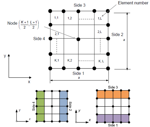
Figure 1. Depiction of the box used in the crown method.

Once the box and the fluxes in each of the points of it are obtained, the following equations are used in order to obtain the bypass and total fluxes.

\[N_{xx}^{bypass} = \left\{ \begin{array}{r} N_{xx}^{side\ 2},\ \ \left| N_{xx}^{side\ 2} \right| \leq \left| N_{xx}^{side\ 4} \right| \ N_{xx}^{side\ 4},\ \ \left| N_{xx}^{side\ 2} \right| \geq \left| N_{xx}^{side\ 4} \right| \ 0,\ \ sgn\left( N_{xx}^{side\ 2} \right) \neq sgn\left( N_{xx}^{side\ 4} \right) \end{array} \right.\ \]

\[N_{yy}^{bypass} = \left\{ \begin{array}{r} N_{yy}^{side\ 1},\ \ \left| N_{yy}^{side\ 1} \right| \leq \left| N_{yy}^{side\ 3} \right| \ N_{yy}^{side\ 3},\ \ \left| N_{yy}^{side\ 1} \right| \geq \left| N_{yy}^{side\ 3} \right| \ 0,\ \ sgn\left( N_{yy}^{side\ 1} \right) \neq sgn\left( N_{yy}^{side\ 3} \right) \end{array} \right.\ \]

\[N_{xy}^{bypass} = \left\{ \begin{array}{r} N_{xy}^{side\ 1},\ \ \left| N_{xy}^{side\ 1} \right| = \min\left( \left| N_{xy}^{side\ 1} \right|,\ \left| N_{xy}^{side\ 2} \right|,\ \left| N_{xy}^{side\ 3} \right|,\ \left| N_{xy}^{side\ 4} \right| \right) \ N_{xy}^{side\ 2},\ \ \left| N_{xy}^{side\ 2} \right| = \min\left( \left| N_{xy}^{side\ 1} \right|,\ \left| N_{xy}^{side\ 2} \right|,\ \left| N_{xy}^{side\ 3} \right|,\ \left| N_{xy}^{side\ 4} \right| \right) \ N_{xy}^{side\ 3},\ \ \left| N_{xy}^{side\ 3} \right| = \min\left( \left| N_{xy}^{side\ 1} \right|,\ \left| N_{xy}^{side\ 2} \right|,\ \left| N_{xy}^{side\ 3} \right|,\ \left| N_{xy}^{side\ 4} \right| \right) \ N_{xy}^{side\ 4},\ \ \left| N_{xy}^{side\ 4} \right| = \min\left( \left| N_{xy}^{side\ 1} \right|,\ \left| N_{xy}^{side\ 2} \right|,\ \left| N_{xy}^{side\ 3} \right|,\ \left| N_{xy}^{side\ 4} \right| \right) \end{array} \right.\ \]

\[M_{xx} = \frac{M_{xx}^{side\ 2} + M_{xx}^{side\ 4}}{2},\ \ M_{yy} = \frac{M_{yy}^{side\ 1} + M_{yy}^{side\ 3}}{2}\]

\[M_{xy} = \frac{M_{xy}^{side\ 1} + M_{xy}^{side\ 2} + M_{xy}^{side\ 3} + M_{xy}^{side\ 4}}{4}\]

However, the method used in this case is more similar to the FastPPH method, as the fluxes in 8 points will be obtained and used.

Figure 2. Box configuration adapted for the FastPPH method.

\[N_{xy}^{side\ 1} = Avg\left( N_{xy}^{k,1},\ N_{xy}^{k,2},\ \ldots,\ N_{xy}^{k,l} \right),\ \ N_{xy}^{side\ 2} = Avg\left( N_{xy}^{1,l},\ N_{xy}^{2,l},\ \ldots,\ N_{xy}^{k,l} \right)\]

\[N_{xy}^{side\ 3} = Avg\left( N_{xy}^{1,1},\ N_{xy}^{1,2},\ \ldots,\ N_{xy}^{1,l} \right),\ \ N_{xy}^{side\ 4} = Avg\left( N_{xy}^{1,1},\ N_{xy}^{2,1},\ \ldots,\ N_{xy}^{k,1} \right)\]

\[M_{xy}^{side\ 1} = Avg\left( M_{xy}^{k,1},\ M_{xy}^{k,2},\ \ldots,\ M_{xy}^{k,l} \right),\ \ M_{xy}^{side\ 2} = Avg\left( M_{xy}^{1,l},\ M_{xy}^{2,l},\ \ldots,\ M_{xy}^{k,l} \right)\]

\[M_{xy}^{side\ 3} = Avg\left( M_{xy}^{1,1},\ M_{xy}^{1,2},\ \ldots,\ M_{xy}^{1,l} \right),\ \ M_{xy}^{side\ 4} = Avg\left( M_{xy}^{1,1},\ M_{xy}^{2,1},\ \ldots,\ M_{xy}^{k,1} \right)\]

Obtention of the box

The first step in the calculation of bypass loads is the obtention of the box that will help define the area where the calculations will be made. This box dimension \(a\) is defined using the following expression:

\[a = 0.4 \times AF \times MF \times d\]

where \(AF\) is the area factor, \(MF\) is the material factor (which is different depending on whether the plate is made out of a metallic material or a composite material) and \(d\) is the diameter.

Knowing its dimension, the box should be defined with a specific orientation and order. The orientation is defined by the box reference frame, which coincides with the material system of the element where the joint is pierced. This may cause a small variation because the z-axis is defined as the joint’s axial direction, and sometimes the material system’s z-axis does not coincide with it.

Then, the box system’s origin would be placed in the center of the box and the first point would be located in (-a, a) and the other points would be placed in the clockwise direction.

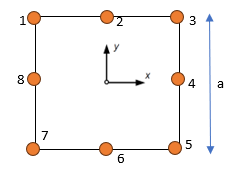
Figure 3. Orientation of the box points.

This does not always coincide with what Altair displays, but the final results should be the same.

Once the box is formed, the next step is to obtain and locate the box points in the model’s geometry, so there are two cases, depending on whether all box points are located within the free edges of the component or not.

Adjacent elements will be evaluated until the distance from the joint to them is greater to the box’s semidiagonal. After this, no more points will be found further away, so the search stops here. If there are still points to be assigned, it is concluded that they lie outside of the edge of the plate and therefore they will be projected.

If all points lie within the free edges, the process is simple. The adjacent elements to the pierced one are evaluated in case that any point lies inside of it, which is done taking into consideration the so-called box tolerance, stopping the iterations when the element that is being analysed is far from the box location.

However, there are two cases where the box point location is not as simple. Firstly, if there are points outside the free edges, they are orthogonally projected onto the mesh. In the FastPPH tool used by Altair, this projection does not always follow the same procedure but, to simplify, in this tool an orthogonal projection is always used.

The second critical case occurs when a box crosses a T-edge (Figure 4) or gets out of a surface that does not finish in a free edge (Figure 5). If the box crosses a T-edge, it is considered that all points are located within the free edges and should not be projected. If the box gets out of the borders of a surface, and these borders are not free edges, they are treated as so, and the same procedure is followed as when they were outside of free edges (they are orthogonally projected).

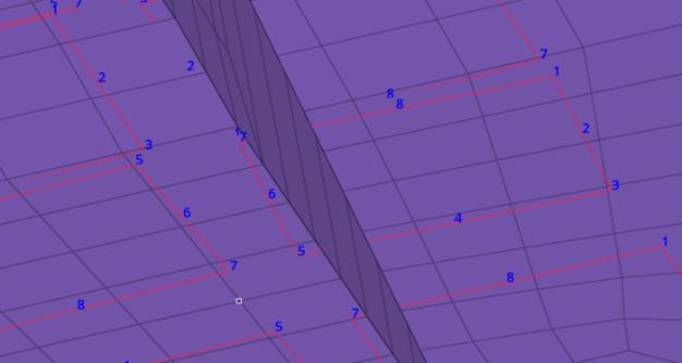
Figure 4. Case of a box crossing a T-edge.

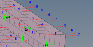
Figure 5. Case of a surface that does not finish in a free edge.

Obtention of the fluxes

Now, the fluxes in each of the points of the boxes, for each load case, must be obtained, in order to calculate the final values for bypass and total loads. There are two options to be analysed:

(a) “cornerData” is set to True

If the user asks for results in the corner when running the model and obtaining the corresponding results, these results will be given by node and not by element, giving several values for a node, related to the element where it is. This can be achieved by selecting the CORNER or BILIN describer in the FORCE card. Results will be more accurate if corner data is used, as there are more values to be used.

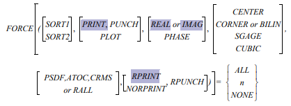
Figure 6. Structure of the FORCE card

Taking each of the box’s points, the same procedure is carried out. Firstly, the results for all nodes that form the element where the box point is are retrieved. They are represented in their element reference frame, so they are transformed into the same reference frame. Once 3 or 4 values for the nodes are obtained (depending on wether the element is a TRIA or QUAD), a bilinear interpolation to the box point from the node locations is used.

Finally, the obtained values for the point are transformed to the material reference frame of the element where the bolt is pierced, which will be the system where the forces are to be represented in.

If the following picture is taken as an example, the calculation of forces in point 2 would be as follows:

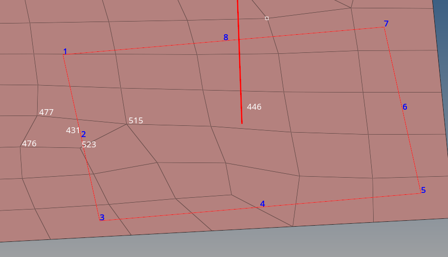
Figure 7. Example of the obtention of fluxes with corner data.

As the point is located in element 431, the forces for the nodes that form it are retrieved, those nodes being the ones with IDs 476, 477, 515 and 523. It can be seen that, for nodes 476 and 477, four values would be obtained, as they are contained in four different elements. However, node 523 would have three values and 515 would have 5 values. Then, all the results should be transformed to be represented in the element reference frame of element 431 to make the average and obtain a single result for each node. Next, an interpolation from the four nodes to the point 2 is done and, finally, the transformation from the element reference frame of element 431 to the material reference frame of element 446 is done.

(b) “cornerData” is set to False

The results in the result files are retrieved in the centroid of each element, leading to results that will be less precise, since results in the corners must be approximated instead of actually calculated. This approximation is made by averaging the adjacent elements. Besides this, the same procedure is used as in the previous case.

Finally, all results are transformed into the material reference frame corresponding to the element where the joint is pierced.

Considering the same example as before:

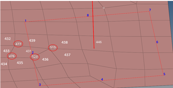
Figure 8. Example of the obtention of fluxes without corner data.

The “goal” is to get the data in the surrounding nodes in order to be able to interpolate and obtain the result in point 2. Thus, if we use as an example node 515, the data in the centroid for elements 439, 431, 436, 437 and 438 should be retrieved. These values should be represented in the same reference frame (element reference frame of element 431). Finally, the average between these values should be computed in order to get the value in the node. This procedure should be carried out for all the nodes of the point element. Once these values have been computed, the same methodology is followed as in the corner data case: interpolate from the corners to the point and transform onto the element reference frame where the bolt is pierced.

Obtention of the bypass and total fluxes

Finally, once the calculation of the fluxes in the box points has been done, the calculation of the total and bypass loads is carried out with the expressions written above. Thus, the first step is to obtain the loads in the sides of the box, which are done by an average using the points of the corresponding side. Once these box sides computation has been done, the expressions for total and bypass loads are used. In a similar way, the bypass maximum and minimum principals are computed with the following formulas:

\[N_{max,\ \ min} = \frac{N_{x} + N_{y}}{2} \pm \sqrt{\left( \frac{N_{x} - N_{y}}{2} \right)^{2} + N_{xy}^{2}}\]

Finally, all results are represented in the material reference frame of the plate where the bolt is pierced. This has been decided to follow this criterion in order to coincide with the exports by Altair.

Final considerations

Several errors could occur, which are related to the following:

• There are less than two plates connected to the analysed joint.

• A plate does not have the necessary information (intersection, normal, distance and elements).

• The joint has no diameter or it is negative.

• The maximum number of iterations is reached.

• There are not enough adjacent elements, which usually means that the adjacency radius is too low. In this case, attributes are filled with zeros.

• There are no candidate elements to search.

• Certain arrays do not have, for whatever reason, six elements.

• The final rotation matrix is not well defined.

Just like in “get_forces”, this process is done for each joint in the model and, after each joint has had its forces calculated, a progress bar is updated showing how many joints have been analysed and how many are remaining.

In N2PGetFasteners, an error will occur if this method is used before the “get_results_joints” one, as well as if there are joints with no diameter. Note that this method can be used before or after the “get_forces” one.

PAG method

The “get_bypass_loads_PAG” method is also located in N2PJoint and has the same inputs, except for the fact that it does not have a box tolerance argument and has the following extra argument:

• incraseTol: float that represents the percentage-wise increase in the tolerance used in the projections. In N2PGetLoadFasters, this input is the value corresponding to the “TOLERANCE INCREMENT” key in the “BypassParameters” attribute.

The main differences between the “get_bypass_loads” method and the “get_bypass_loads_PAG” one are:

• In the latter method, the obtention of the box and the rest of the calculations are located in N2PPlate, under the “get_box_PAG” and “get_bypass_PAG” names, while in the former method, all of the calculations were done in N2PJoint.

• The total momentums \(M_{xx}\), \(M_{yy}\) and \(M_{xy}\) are not the average of the momentum fluxes in their corresponding sides, but the maximum value of the fluxes (in absolute value).

• The algorithm used in the obtention of the box is slightly altered, but the theory behind it is the same.

Results export

Finally, results could be exported by using the “export_results” method (which is located in N2PGetLoadFasteners and has no inputs or outputs). Depending on what the TypeExport attribute is, the results are exported in a different way.

Altair, NaxToPy or PAG CSV style

If results are to be exported in the Altair, NaxToPy or PAG_CSV style, they are exported by calling the “export_forces” method, which is located in N2PJoints and has the following inputs:

• model: N2PModelContent object defining the model. In N2PGetLoadFasteners, this input is its “Model” attribute.

• pathFile: string which represents where the CSV file is to be created. In N2PGetLoadFasteners, this input is its “ExportLocation” attribute.

• analysisName: string which represents the name of the CSV file that is generated.

• results: dictionary which represents the results obtained previously. In N2PGetLoadFasteners, this input is its “Results” attribute.

• typeExport: string which represents the way that results are to be exported. In N2PGetLoadFasteners, this input is its “TypeExport” attribute.

This method has no outputs and it simply extracts information from its inputs and transforms it in a way that makes it comfortable to export. If “typeExport” is set to “NAXTOPY”, the generated CSV has the following columns:

• Bolt ID: ID of the analysed bolt/joint.

• Plate Global ID: global ID of the analysed plate.

• Plate Local ID: internal ID of the analysed plate.

• Plate Element ID: solver ID of the central element associated to the plate.

• Plate Element Property ID: ID of the N2PProperty associated to the previous element.

• Bolt Element 1 ID: solver ID of the first element associated to the bolt.

• Bolt Element 2 ID: solver ID of the second element associated to the bolt. If there is no second element, ‘0’ is displayed instead.

• Load Case ID: ID of the analysed load case.

• Analysis Name: analysis name as defined by the user.

• Box Dimension: dimension of the box used in the bypass loads calculation.

• Box System: reference frame of the previous box.

• Intersection: intersection point between the plate and its bolt.

• FX Altair, FY Altair, FZ Altair: 1D forces as calculated by Altair.

• FX Connector 1, FY Connector 1, FZ Connector 1, FX Connector 2, FY Connector 2, FZ Connector 2: 1D forces of each of the elements that make up the bolt.

• FZ max: bolt’s maximum axial force.

• p1, p2, …, p8: global coordinates that define the box.

• Fxx p1, Fxx p2, …, Fxx p8: Fxx flux associated to the points that define the box.

• Fyy p1, …: Fyy flux associated to the points that define the box.

• Fxy p1, …: Fxy flux associated to the points that define the box.

• Mxx p1, …: Mxx flux associated to the points that define the box.

• Myy p1, …: Myy flux associated to the points that define the box.

• Mxy p1, …: Mxy flux associated to the points that define the box.

• Nx bypass, Nx total, Ny bypass, Ny total, Nxy bypass, Nxy total, Mx total, My total, Mxy total: bypass loads, total loads and total moments calculated in each axis.

If “typeExport” is set to “ALTAIR”, the generated CSV will have the following columns:

• DDP: ID of the analysed bolt/joint.

• elementid: solver ID of the central element associated to the plate.

• Component Name: name of the element’s property.

• elem 1 id: solver ID of the first element associated to the bolt.

• elem 1 node id: solver ID of the first node associated to the first bolt element.

• elem 2 id: solver ID of the second element associated to the bolt. If there is no second element, ‘0’ is displayed instead.

• elem 2 node id: solver ID of the first node associated to the second bolt element. If there is no second element, ‘0’ is displayed instead.

• box dimension: dimension of the box used in the bypass loads calculation.

• loadcase: ID of the analysed load case.

• file name: analysis name as defined by the user.

• LoadCase Name: name of the analysed load case.

• Time Step Name: “N/A” is displayed.

• pierced location: intersection point between the plate and its bolt.

• FX, FY, FZ: 1D forces as calculated by Altair.

• p1, p2, …, p8: global coordinates that define the box.

• Fxx p1, Fxx p2, …, Fxx p8: Fxx flux associated to the points that define the box.

• Fyy p1, …: Fyy flux associated to the points that define the box.

• Fxy p1, …: Fxy flux associated to the points that define the box.

• Mxx p1, …: Mxx flux associated to the points that define the box.

• Myy p1, …: Myy flux associated to the points that define the box.

• Mxy p1, …: Mxy flux associated to the points that define the box.

• Nx bypass, Nx total, Ny bypass, Ny total, Nxy bypass, Nxy total, Mx total, My total, Mxy total: bypass loads, total loads and total moments calculated in each axis.

If “typeExport” is set to “PAG_CSV”, the generated CSV will have the following columns:

• PLATE ELEMENT ID: solver ID of the central element associated to the plate.

• LOAD CASE ID: ID of the analysed load case.

• PROPERTY: property of the analysed plate.

• CFAST A ID, CFAST B ID: solver ID of the A and B CFASTs. If there is no A or B CFAST, ‘0’ is displayed instead.

• DIRECTION: combination of the direction of both CFASTs in the plate.

• GA NODE CFAST A, GB NODE CFAST A, GA NODE CFAST B, GB NODE CFAST B: solver ID of the nodes associated to each CFAST. If there is no A or B CFAST, ‘0’ is displayed instead.

• DIAMETER: diameter of the analysed joint.

• EXT. ZONE: shape of the bypass box.

• ELEMENT 1 ID, …, ELEMENT 8 ID: solver ID of the elements in which each point of the bypass box is located.

• POINT 1 (X, Y, Z), …, POINT 8 (X, Y, Z): coordinates of each point of the bypass box.

• X BEARING FORCE, Y BEARING FORCE, PULLTHROUGH FORCE: each of the three coordinates of the bearing force of the plate.

• BOLT SHEAR: shear force of the plate.

• BOLT TENSION: maximum axial force of the plate.

• NXX BYPASS, NYY BYPASS, NXY BYPASS, MXX BYPASS, MYY BYPASS, MXY BYPASS: bypass forces and momentums.

• FXX CFAST A, FYY CFAST A, FZZ CFAST A, …, FZZ CFAST B: forces of each fastener associated to the plate.

• FXX POINT 1, FYY POINT 1, FXY POINT 1, MXX POINT 1, MYY POINT 1, MXY POINT 1, …, MXY POINT 8: force and momentum fluxes of each point in the bypass box.

• FXX NORTH, FYY NORTH, FXY NORTH, MXX NORTH, MYY NORTH, MXY NORTH, …, MXY WEST: force and momentum fluxes of each side of the bypass box.

In N2PGetFasteners, an error will occur if this method is used before the “get_forces_joints” or “get_bypass_joints” one. In N2PJoint, an error will occur if the “TypeExport” attribute is not “NAXTOPY”, “ALTAIR” or “PAG_CSV”.

PAG TXT style

If results are to be exported in the PAG_TXT style, they are exported by calling the “__export_pag_txt” method, which is located in N2PGetLoadFasteners and has no inputs or outputs. It generates six sections of data with the following information.

In the first section, the following columns are written:

• A/B-ELEM: solver ID of the central element associated to the plate.

• A/B-PROPERTY: property of the analysed plate.

• CFAST_A, CFAST_B: solver ID of the A and B CFASTs. If there is no A or B CFAST, ‘0’ is displayed instead.

• DIRECTIONS: combination of the direction of both CFASTs in the plate.

• EXT. ZONE: shape of the bypass box.

• ELEMENT_1, …, ELEMENT_8: solver ID of the elements in which each point of the bypass box is located.

• POINT_1(X,Y,Z), …, POINT_8(X,Y,Z): coordinates of each point of the bypass box.

In the first section, the following columns are written:

• CFAST-ID: solver ID of each fastener.

• CFAST-PROPERTY: property of the analysed fastener.

• GS-NODE, GA-NODE, GS-NODE: GA, GB and GS nodes of the analysed fastener.

• A-ELEM, B-ELEM: solver ID of the “A” and “B” elements of the analysed fastener.

• DIAM(mm): diameter of the analysed joint.

• MATERIAL: material of the plates attached to the fastener.

In the third section, called “RESULTS”, the following columns are written:

• A/B-ELEM: solver ID of the central element associated to the plate.

• A/B-PROPERTY: property of the analysed plate.

• LOADCASE,SUBCASE: string of the ID and name of the analysed load case.

• BypassFlux Nxx(N/mm), BypassFlux Nyy(N/mm), BypassFlux Nxy(N/mm): bypass forces.

• XBearing Force(N), YBearing Force (N), PullThrough Force (N): bearing forces.

• TotalMomentum Flux_Mxx(N), TotalMomentum Flux_Myy(N), TotalMomentum Flux_Mxy(N): bypass momentums.

• BoltShear Force(N): shear force of the plate.

• BoltTension Force(N): maximum axial force of the plate.

In the fourth section, called “TRANSLATIONAL_FASTENER_FORCES”, the following columns are written:

• A/B-ELEM: solver ID of the central element associated to the plate.

• A/B-PROPERTY: property of the analysed plate.

• LOADCASE,SUBCASE: string of the ID and name of the analysed load case.

• CFAST_A Fxx(N/mm), CFAST_A Fyy(N/mm), CFAST_A Fxy(N/mm), …, CFAST_B Fxy(N/mm): forces of each fastener associated to the plate.

• CFAST_A Factor(-), CFAST_B Factor(-): CFAST factor of each fastener.

In the fifth section, called “EXTRACTION_POINT_SHELL_FORCE_FLUXES”, the following columns are written:

• A/B-ELEM: solver ID of the central element associated to the plate.

• A/B-PROPERTY: property of the analysed plate.

• LOADCASE,SUBCASE: string of the ID and name of the analysed load case.

• POINT_1 Fxx(N/mm), POINT_1 Fyy(N/mm), POINT_1 Fxy(N/mm), …, POINT_8 Fxy(N/mm): force fluxes of each point of the bypass box.

• AVG_NORTH Fxx(N/mm), AVG_NORTH Fyy(N/mm), AVG_NORTH Fxy(N/mm), …, AVG_EAST Fxy(N/mm): force fluxes of each side of the bypass box.

• BYPASS Fxx (N/mm), BYPASS Fyy (N/mm), BYPASS Fxy (N/mm): bypass forces.

In the sixth section, called “EXTRACTION_POINT_SHELL_MOMENTUM_FLUXES”, the following columns are written:

• A/B-ELEM: solver ID of the central element associated to the plate.

• A/B-PROPERTY: property of the analysed plate.

• LOADCASE,SUBCASE: string of the ID and name of the analysed load case.

• POINT_1 Mxx(N), POINT_1 Myy(N), POINT_1 Mxy(N), …, POINT_8 Mxy(N): momentum fluxes of each point of the bypass box.

• AVG_NORTH Mxx(N), AVG_NORTH Myy(N), AVG_NORTH Mxy(N), …, AVG_EAST Mxy(N): momentum fluxes of each side of the bypass box.

• BYPASS Mxx (N), BYPASS Myy (N), BYPASS Mxy (N): bypass momentums.

PAG HDF5 style

If results are to be exported in the PAG_TXT style, they are exported by calling the “__export_pag_hdf5” method, which is located in N2PGetLoadFasteners and has no inputs or outputs. It generates an HDF5 with the “create_dataset” function and writes all necessary information with the “write_dataset” function. The information written is the one obtained in “get_forces_joints” and “get_bypass_joints”, and is adequately transformed in the “__transform_results” method, which is located in N2PGetLoadFastener and has the following inputs:

• loadcase: integer representing the ID of the load case to be analysed.

• p: N2PPlate instance representing the plate whose information is to be exported.

It has the following output:

• dataEntry: DataEntry instance which will be the input of the “write_dataset” function.

The following information will be written:

• ID_ENTITY: solver ID of the analysed plate.

• BYPASS FLUX NXX, BYPASS FLUX NYY, BYPASS FLUX NXY: bypass forces.

• X BEARING FORCE, Y BEARING FORCE, PULLTHROUGH FORCE: bearing forces.

• TOTAL MOMENTUM FLUX MXX, TOTAL MOMENTUM FLUX MYY, TOTAL MOMENTUM FLUX MXY: bypass momentums.

• BOLT SHEAR: shear force of the bolt associated to the analysed plate.

• BOLT TENSION: maximum axial force of the bolt associated to the analysed plate.

• FXX CFAST A, FYY CFAST A, FXY CFAST A, …, FXY CFAST B: translational fastener forces of each fastener associated to the plate.

• FXX POINT 1, …, MXY POINT 1, …, MXY POINT 8: bypass fluxes of each point of the bypass box.

• FXX NORTH, …, MXY EAST: bypass fluxes of each side of the bypass box.

All this information is expressed as an array with a predetermined data type, whose names are the ones shown above and its type is a float of a certain precision, as determined by the user in the ExportPrecision attribute, or an integer (just for ID_ENTITY). This array is the Data attribute of dataEntry. Other attributes which are also filled in are:

• ResultsName: “FASTENER ANALYSIS”.

• LoadCase: the “loadcase” input of this method.

• Section: “NONE”.

• PartName: the part ID of the first element in the plate.

N2PGetLoadFastener calculation

While the user could perfectly call all of the aforementioned methods individually, this may not be practical. By using the “get_analysis_joints” method (which is located in N2PGetLoadFasteners and has no inputs or outputs), the “get_forces_joints” and “get_bypass_joints” methods are called. Furthermore, by using the “calculate” method, the “get_results_joints” and “get_analysis_joints” methods are called, and, if the “ExportLocation” attribute has been set, the “export_results” method is also called.

Auxiliary functions

During the program, some auxiliary functions are used. These functions are located in N2PInterpolation and N2PRotation.

N2PInterpolation

The functions located in N2PInterpolation obviously are related to interpolation, which is necessary to calculate the bypass loads. The following functions are used:

Transformation to isoparametric coordinates

One of the most important things when interpolating is having a correct representation of the element that is been used. Thus, the shape functions are crucial in this step. The function called “transform_isoparametric” transforms a 3D point to isoparametric coordinates within a quadrilateral. It has the following inputs:

• point: list or Numpy array of three floats with the coordinates of the point.

• quad: list of four 3D points defining the quads.

• tol: float that represents the tolerance value. By default, it is set to 0.01.

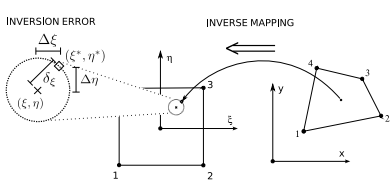
Figure 9. Procedure carried out by the function.

This function’s outputs are the isoparametric coordinates \(\xi\) and \(\eta\) of the point within the quad.

The procedure is based on the following expressions:

\[x = a_{0} + a_{1}\xi + a_{2}\eta + a_{3}\xi\eta,\ \ y = b_{0} + b_{1}\xi + b_{2}\eta + b_{3}\xi\eta\]

\[\xi = \frac{x - a_{2}\eta}{a_{1} + a_{3}\eta},\ \ A\eta^{2} + B\eta + C = 0 \Rightarrow \left\{ \begin{array}{r} A = a_{3}b_{2} - a_{2}b_{3} \ B = \left( b_{3}x + a_{1}b_{2} \right) - \left( a_{3}y + a_{2}b_{1} \right) \ C = b_{1}x - a_{1}y \end{array} \right.\ \]

\[a_{0} = \frac{\left( x_{n}^{1} + x_{n}^{2} \right) + \left( x_{n}^{3} + x_{n}^{4} \right)}{4},\ \ b_{0} = \frac{\left( y_{n}^{1} + y_{n}^{2} \right) + \left( y_{n}^{3} + y_{n}^{4} \right)}{4}\]

\[a_{1} = \frac{\left( x_{n}^{2} - x_{n}^{1} \right) + \left( x_{n}^{3} - x_{n}^{4} \right)}{4},\ \ b_{1} = \frac{\left( y_{n}^{2} - y_{n}^{1} \right) + \left( y_{n}^{3} - y_{n}^{4} \right)}{4}\]

\[a_{2} = \frac{\left( x_{n}^{3} + x_{n}^{4} \right) - \left( x_{n}^{1} + x_{n}^{2} \right)}{4},\ \ b_{2} = \frac{\left( y_{n}^{3} + y_{n}^{4} \right) - \left( y_{n}^{1} + y_{n}^{2} \right)}{4}\]

\[a_{4} = \frac{\left( x_{n}^{1} - x_{n}^{2} \right) + \left( x_{n}^{3} - x_{n}^{4} \right)}{4},\ \ b_{4} = \frac{\left( y_{n}^{1} - y_{n}^{2} \right) + \left( y_{n}^{3} - y_{n}^{4} \right)}{4}\]

Some other considerations about the shape of the quadrilateral must be taken into account when applying these expressions.

Transformation to barycentric coordinates

In a similar way as in the previous section, the function “transform_barycentric” transform a 3D point to barycentric coordinates within a triangle. This function has as inputs:

• point: list or Numpy array of three floats with the coordinates of the point.

• nodes: list of three 3D points defining the triangle.

This function’s outputs are the barycentric coordinates \(\alpha\), \(\beta\) and \(\gamma\) of the point within the triangle. These coordinates are obtained solving the following linear system of equations:

\[\left\{ \begin{array}{r} x = \alpha x_{A} + \beta x_{B} + \gamma x_{C} \ y = \alpha y_{A} + \beta y_{B} + \gamma y_{C} \ 1 = \alpha + \beta + \gamma \end{array} \right.\ \]

Interpolation

Once the previous transformations have been done, the interpolation of the forces onto the box is done by using the function “interpolation”. This function has as inputs:

• point: 1D ndarray of shape (3,) representing the 3D point in the shape.

• vertices: 2D ndarray of shape (n, 3) representing the coordinates of the element corners (n = 3 for a triangle and n = 4 for a quadrilateral).

• values: 2D ndarray of shape (n, 6) representing the forces at the corners.

Its output is a 1D ndarray of shape (6,), which is the force in the desired point after having interpolated. For a triangle, the procedure is the following:

\[F_{I} = \alpha F_{1} + \beta F_{2} + \gamma F_{3}\]

where \(F_{I}\) is the interpolated force and \(F_{N}\) is the force in the \(N\)th corner. For a quadrilateral, the procedure is the following:

\[f_{00} = \frac{F_{1}(1 - u)(1 - v)}{4},\ \ f_{01} = \frac{F_{2}(1 + u)(1 - v)}{4}\]

\[f_{10} = \frac{F_{3}(1 + u)(1 + v)}{4},\ \ f_{11} = \frac{F_{4}(1 - u)(1 + v)}{4}\]

\[F_{I} = f_{00} + f_{01} + f_{10} + f_{11}\]

N2PRotation

The functions located in N2PRotated obviously are related to the rotation and transformation of forces from one coordinate system to another. The following functions are used:

Tensor rotation

Matrices, or 2D tensors, can be rotated using the “rotate_tensor2D” function. Its inputs are:

• fromSystem: list or ndarray representing the reference frame where the tensor is represented.

• toSystem: list or ndarray representing the reference frame where the tensor is to be represented.

• planeNormal: list or ndarray representing the rotation plane.

• tensor: list or ndarray representing the tensor to be rotated.

The function’s output is the rotated tensor.

Vector rotation

Vectors can be rotated using the “rotate_vector” function. Its inputs are:

• vector: list or ndarray representing the vector to be rotated. Its size must be proportional to three.

• fromSystem: list or ndarray representing the reference frame where the vector is represented.

• toSystem: list or ndarray representing the reference frame where the vector is to be represented.

The function’s output is the rotated vector.

Vector projection

Vectors can be projected using the “project_vector” function. Its inputs are:

• vector: list or ndarray representing the vector to be projected. Its size must be proportional to three.

• fromSystem: list or ndarray representing the reference frame where the vector is projected.

• toSystem: list or ndarray representing the reference frame where the vector is to be projected.

The function’s output is the projected vector.

Angle between two systems

In order to obtain the angle between two reference frames, the “angle_between_2_systems” function is used. Its inputs are:

• fromSystem: list or ndarray representing the first reference.

• toSystem: list or ndarray representing the second reference.

• planeNormal: rotation plane.

The function’s output is the angle between both systems, in radians.

Transformation of a system to a matrix

In order to transform a reference frame given by a list or array of nine components into a \(3 \times 3\) matrix, the “sysToMat” function is used. Its input is:

• system: list of floats representing the reference frame.

The function’s output is the \(3 \times 3\) matrix.

Matrix multiplication

In order to multiply several matrices together without having to use the “np.matmul” function repeatedly, the “matMul” function is used. Its input is:

• matrices: list of arrays representing several matrices of the same size.

The function’s output is the matrix obtained after multiplying all of the matrices in the input.

Determine if a point is inside of an element

In order to determine if a point (given its coordinates) is inside an N2PElement, the “point_in_element” function is used. Its inputs are:

• point: array representing the coordinates of the point.

• element: N2PElement in which the point may be.

• tol: float representing the accepted tolerance, which is 0.01 by default.

The function’s output is simply a True or False Boolean. This is done by using the “point_in_quad” or “point_in_tria” functions, depending on the type of element. Only CQUAD4 and CTRIA3 elements are accepted.

Determine if a point is inside a CQUAD4 element

In order to determine if a point (given its coordinates) is inside a CQUAD4 element, the “point_in_quad” function is used. Its inputs are:

• point: array representing the coordinates of the point.

• element: N2PElement in which the point may be.

• tol: float representing the accepted tolerance, which is 0.01 by default.

The function’s output is simply a True or False Boolean. This is done by splitting the quad in two triangles and determining if a point is inside either of them, which is done using the “point_in_tria” function.

Determine if a point is inside a triangle

In order to determine if a point (given its coordinates) is inside a CTRIA3 element, or a triangle whose vertices are known, the “point_in_tria” function is used. Its inputs are:

• point: array representing the coordinates of the point.

• p1: array representing the coordinates of the first vertex.

• p2: array representing the coordinates of the second vertex.

• p3: array representing the coordinates of the third vertex.

• element: N2PElement in which the point may be.

• tol: float representing the accepted tolerance, which is 0.01 by default.

The function’s output is simply a True or False Boolean. If the element is given, then its vertices are extracted. After the coordinates of the vertices are known, the “barycentric_coords” function is called. If all barycentric coordinates are positive, and its sum is equal to one (within the given tolerance), it is determined that the point is inside the triangle.

Barycentric coordinates

In order to obtain the barycentric coordinates of a point within a triangle, the “barycentric_coords” function is used. Its inputs are:

• point: array representing the coordinates of the point.

• a: array representing the coordinates of the first vertex.

• b: array representing the coordinates of the second vertex.

• c: array representing the coordinates of the third vertex.

The function’s outputs are the barycentric coordinates, which are given by:

\[\alpha = \frac{A_{PCB}}{A_{ABC}},\ \ \beta = \frac{A_{PCA}}{A_{ABC}},\ \ \gamma = \frac{A_{PBA}}{A_{ABC}}\]

where \(A_{XYZ}\) is the area formed by the triangle with X, Y and Z vertices. This function is similar to the “transform_barycentric” function in N2PInterpolation, but the way to obtain the coordinates is slightly altered. To obtain the barycentric coordinates of a point inside a triangle, both are valid, but this one works well to obtain the barycentric coordinates of a point that does not lie within a triangle, as one of the coordinates may be greater than one.

Transformation for interpolation

The “transformation_for_interpolation” function is used to ease the interpolation in the obtention of bypass loads. It transforms the nodes of an element and a point in it from the global reference frame to the element reference frame. Its inputs are:

• cornerPoints: ndarray with the nodes of the element to be transformed.

• centroid: ndarray with the coordinates of the element’s centroid.

• point: ndarray with the coordinates of the point to be transformed.

• elementSystem: ndarray with the element reference frame.

• globalSystem: ndarray with the global reference frame. By default, it is the identity matrix.

References

• JointLoad Method: https://2023.help.altair.com/2023/hwdesktop/hwx/topics/pre_processing/aerospace/methods_built_in_libraries_jointload_r.htm

• hal-00122640v2: Gustavo Silva, Rodolphe Le Riche, Jérôme Molimard, Alain Vautrin. Exact and efficient interpolation using finite elements shape functions. 2007.

---

© 2025 Idaero Solutions S.L. All rights reserved.

This document is licensed under the terms of the LICENSE of the NaxToPy package.